5 Handy Tips for Preparing your Forecasts in Excel.

As an accountant by trade I can sometimes feel like a duck out of water in the world of digital marketing, but luckily for me, we can all appreciate some handy tips when it comes to preparing forecasts and models in Excel.

Now this isn’t all about fancy formulas and shortcuts (although I’ve thrown some in for good measure) but rather a few tips that will help improve the useability and functionality of your forecast while helping you get the job done faster.

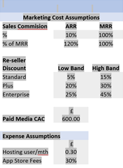
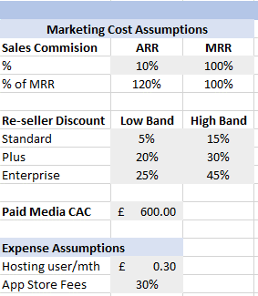
Tip 1 – Include a dedicated section or sheet in your document that lists out all the relevant inputs and assumptions that will drive your forecast.

This small detail can make life a lot easier in a few ways:

• Anyone who needs to review or use the model can quickly see the key assumptions applied in the forecast all in one go and without having to go through multiple sheets.
• All formulas utilising the same inputs can be driven from a single source. This ensures consistency across the model and reduces the risk of errors or miscalculations.

It makes for a more dynamic forecast as inputs and assumptions can easily be updated across the workbook by changing the number in one place only. This allows you to quickly and easily test varying assumptions in your forecast…no updating individual sheets or formulas going on here.

Tip 2 – Use formatting strategically to help others (and yourself) read and use the forecast.

Now you can tackle this in a number of ways and everyone has their own preferences, but two pieces of formatting I would consider in any model are:

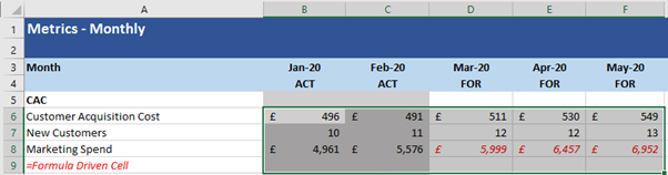
a. The use colour formatting to distinguish between ‘actual’ numbers as opposed to ‘forecast’ numbers.

For example:

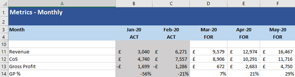
This can be done simply by using Excel’s conditional formatting functionality:

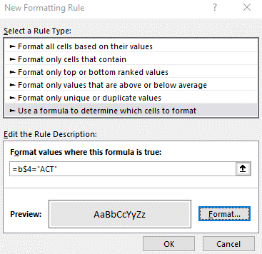
You should note that in the command I have locked the row (‘$4’) but not the column (‘b’) this allows you to copy the formatting across cells and be sure that the format is based on the correct cell.

b. Use formatting to distinguish between cells that contain hardcoded data compared to those containing a formula.

Generally, in a forecast we want to minimise the use of hardcoded data as this can be inefficient to update and lead to errors. However, this is sometimes unavoidable so having a way to quickly identify these cells can save a lot of time and make it easier for others to follow.

For example:

Again, we can utilise conditional formatting to highlight these cells using the ‘=ISFORMULA’ function.

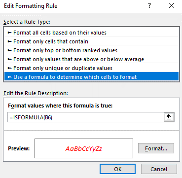
Note: to apply the formatting to the full range you need to select all the relevant cells before navigating to the ‘Conditional Formatting’ command. When entering the ISFORMULA formula you need to refer to the active cell (in this case B6).

Tip 3 – You can group, but you can’t hide

Hidden cells can be a nightmare in any document, particularly if they include data that is being utilised in your forecast. If you have a need to reduce or simplify the information in your model, I strongly recommend the ‘Group’ function in Excel.

This allows you to achieve the same aesthetic appeal of hiding cells without the other complications:

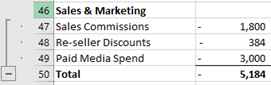
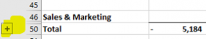
Grouping allows you to quickly identify any summarised information and provides you with a button to shrink and expand the cells.

You can group columns/rows in Excel by selecting the relevant cells and then selecting ‘Group’ containted in the ‘Data’ Toolbar (Shift + Alt + Right is the shortcurt to group or Shift + Alt + Left to ungroup ).

Tip 4 – Use some of Excel’s newer formulas to simply your source data.

Here at Found. we utilise data to drive everything we do, and forecasting is no exception so here are a few handy formulas to help organise and simply your data.

• =UNIQUE – this formula will return only the unique values from a given range (think of the ‘remove duplicates’ button but without the hassle)

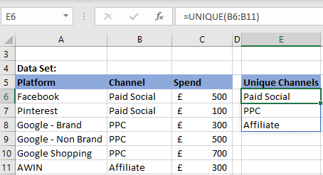
The list of unique channels and is now dynamic and will update as you add or remove additional channels (so long as they appear in the selected range, ‘B6:B11’ in this example).

• =FILTER – this formula will allow you to filter a range with a given criteria (think of the standard ‘filter’ function in excel but as a formula)

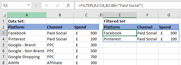
Here we have filtered the data where the value in column B is equal to “Paid Social”.

Tip 5 – Why have one when you could have two?

When you are working on a forecast with multiple sheets it can become tiresome having to switch back and forth, particularly if you need to refer to cells across sheets.

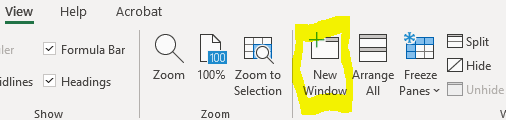
One quick and easy solution to this problem is to create a ‘New Window’ (from within the ‘View’ Toolbar, see below) which will allow you to have one or more copies of the same document open at any given time.

These are simply additional ‘Windows’ of the same Excel document (as opposed to different versions) and so changes in one Window we be updated live in all Windows. This can be very powerful and increase your efficiency, particularly when combined with multiple computer monitors.