Is this the Most Powerful Excel Formula in Digital Marketing?

The formulas & functions in Excel give you the power to get mountains of work done in minimal time. The most powerful formulas of all can do the work of many people at once and save days of campaign time. When it comes to these formulas in my experience of digital marketing, the heavyweight champion is the keyword grouping formula:

=LOOKUP(2^15,SEARCH(C2:C4,A2),D2:D4)
=LOOKUP(2^15,SEARCH(text to look for in your keyword, your keyword), what to return if the text was found)

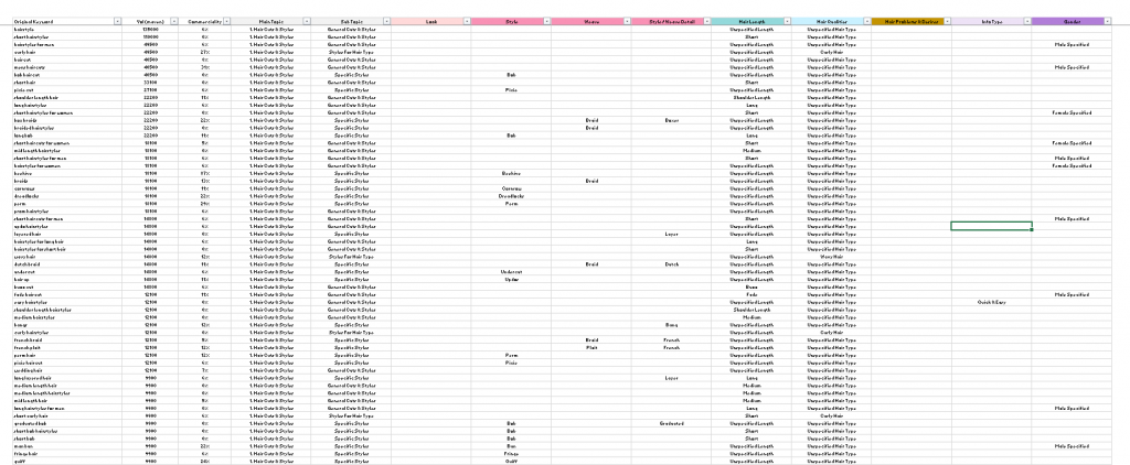
It puts all your millions of keywords into groups based on the words they contain:

But before we unpack it further, let’s dive into an SEO example of why this little monster packs such a punch in the realm of getting stuff done.

SEO is too much work

At the start of a typical SEO campaign we make a Search Landscape document. It’s like a bible for how many people are searching in a vertical (e.g. fashion) and what search terms they are using. Knowing this, we can recommend a site design to our clients which can capture these searches, with landing pages created and / or promoted for each topical area of the vertical where there is sufficient search volume to go to the trouble of making a high quality page e.g. blue shirts.

Sounds like a good plan. Trouble is:

1. We need to know where to draw the line on the pages to be created because we can’t make a page for everything based on limited budgets and the technical problems that come with having too many pages.

2. To know where to draw that line, we need to know how much search volume there is for each topic which could be a potential landing page or new priority.

3. To know that, we need to actually divide the keywords into these topics which could potentially be the focus of a new landing page or priority action.

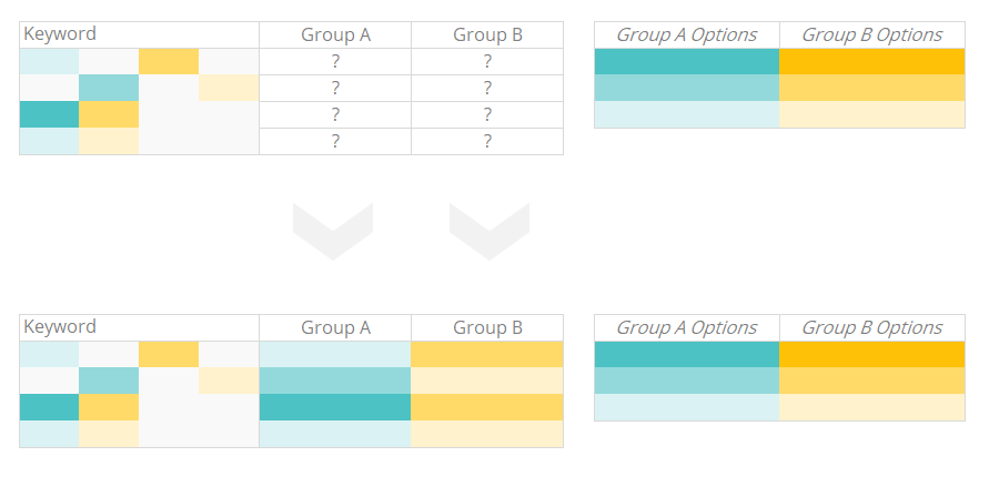
We need something like this:

That’s not that exciting, but what it really gives us is the ability to do this:

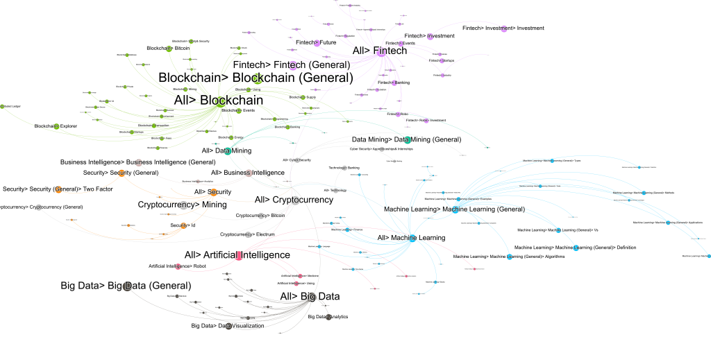
I’ll write another post explaining how to make these visualisations – they require logical and hierarchical keyword grouping, but they let you see the priorities at a glance and you and the client can sit down in a room, point to things on it and treat it like a battle plan.

So to do SEO properly we need to divide keywords into topics, maybe thousands and thousands of them. And it is a complete and utter b*@!ache. Why?

1. Language is messy, synonyms are used all over the place, so there’s often no one word which is shared by all the keywords belonging in a single group and you have to search for multiple synonyms just to organise one group.

2. There isn’t any sufficiently powerful made-for-purpose platform which is really designed to make this easy at large scale – the closest intuitive solution for most Excel users is repeatedly using Excel’s filter option and manually tagging the keywords with their topic. We’ve lost a lot of good souls to this process.

So that’s the problem laid out. For big verticals, it’s too much work for one person. We basically need a team of people grouping the keywords. About now would be a good time for the heroic keyword grouping formula to show up.

 

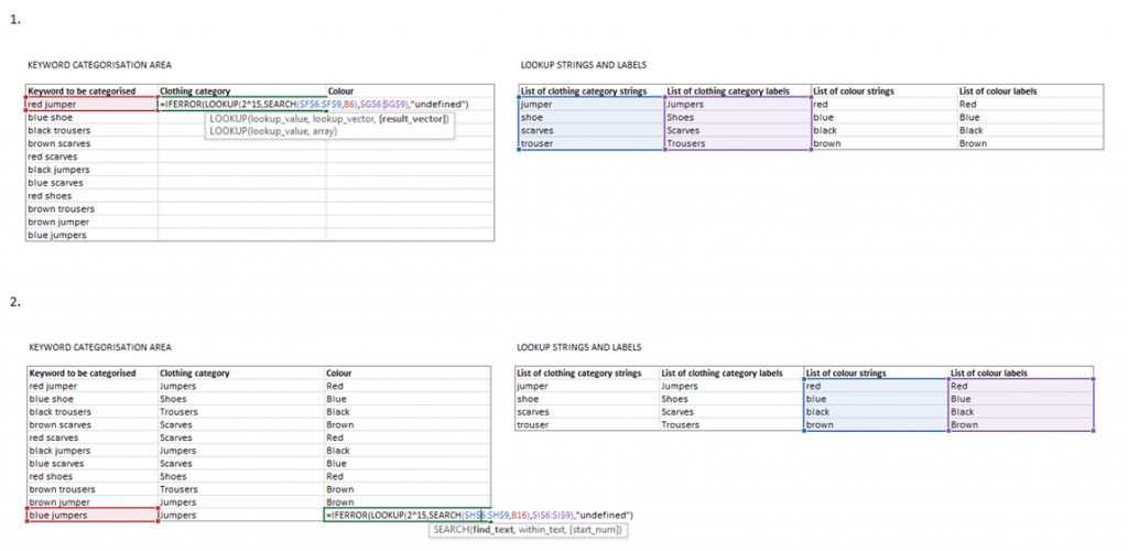
How to use the formula

It’s not the simplest formula to learn – slightly harder than VLOOKUP in my estimation. But when weighed against its power, it is a furiously efficient formula:

=LOOKUP(2^15,SEARCH($C$2:$C$4,A2),$D$2:$D$4)
=LOOKUP(2^15,SEARCH(text to look for in your keyword, your keyword), what to return if the text was found)

How to fill in the parts of the formula:

• $C$2:$C$4 is the text to look for in your keyword which indicates the group it should belong to (alternatively, the list of all the possible words you want to check for in the keyword)
• $D$2:$D$4 is what you want the formula to return if the text was found, it has to be in the same order as the previous range (this can just be the word you’re checking for if you want – same range as above can be used)
• A2 is the cell containing the keyword phrase which you are searching to see if it contains any of the listed strings so you can label it as such with what is returned from the range above.

Other things to know:

• I usually put an IFERROR around the formula to return something nice & tidy when no match is found, rather than an error.
• The formula reads your list of words to search for from the bottom up. So if you want to group the keyword ‘light blue shirt’ and you have colour options for ‘blue’ and ‘light blue’, make sure ‘light blue’ is lower down the list than ‘blue’ – this will ensure that the formula returns a match for ‘light blue’ rather than the less-accurate ‘blue’. In short – put longer, more detailed words to search for lower down in your list.

So you make the formula, drag it down and it categorises your keywords, doing the work of many people in seconds.

Have no illusions – if your keyword list is big, you’ll still need to do a lot of work to clean up the output, but you just saved many expensive and tedious hours.

 

The Brilliance of how this Formula works

The remarkable thing about this formula is that it takes an unlikely combination of functions to do something for which Excel was never intended, brilliantly well.

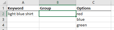
Let’s say we want to find out which colour category a keyword belongs in. We have a spreadsheet laid out like this, and want the result of the formula in B2 to be the group ‘blue’:

Here’s the formula again:

=LOOKUP(2^15,SEARCH($C$2:$C$4,A2),$D$2:$D$4)
=LOOKUP(2^15,SEARCH(text to look for in your keyword, your keyword), what to return if the text was found)

Now we’re going to take it apart and re-build it, step by step. Let’s ignore the IFERROR and concentrate on the 2 core functions, starting from the middle.

 

FUNCTION #1: SEARCH

SEARCH returns the starting location of a text string inside another text string:

=SEARCH(find_text, within_text)
=SEARCH(get the position number of the start of this, within this)

For example, the SEARCH formula below returns ‘4’ because ‘def’ begins from the 4th character in ‘abcdef’:

=SEARCH("def","abcdef")

Nice & simple.

SEARCH is a great way of telling if something is in something else, which is the core purpose of what we’re trying to do. If it brings back a number, we know what we’re looking for is in there.

But in our grouping formula, find_text isn’t a single value or cell reference – it’s a range of cells. So let’s try that now, but with SEARCH on its own, with C2:C4 as colour categories ‘red,’ blue’, ‘green’ and A2 as the keyword ‘light blue shirt’:

=SEARCH(C2:C4,A2)

If this worked like before, we’d expect to get a ‘7’ as the result because matching ‘blue’ starts at position 7 in the keyword. Instead we get a #VALUE! error because the search function doesn’t take ranges – at least not on its own. It’s too narrow minded. It needs a friend to loosen it up a little.

 

FUNCTION #2: LOOKUP

There’s a reason you haven’t used it before. It’s like VLOOKUP’s ne’er-do-well brother who has lucked out with a better name. But it turns out that LOOKUP was born with an obscure special talent, like a world championship skill level at tiddlywinks or playing the digeridoo:

When lookup_value (what we’re looking for) is greater than all values in lookup_vector (where we’re looking for it) and therefore cannot be found, LOOKUP matches the last non-error value in lookup_vector.

=LOOKUP(lookup_value, lookup_vector)
=LOOKUP(what we're looking for, where we're looking for it)
=LOOKUP(2^15, C2:C4)

Don’t expect to get this just yet. All you need to know for now is that it just so happens that this ability of LOOKUP to bring back the last non-error value of its lookup range when the lookup value can’t be found is exactly what we need.

The lookup_value we are going to use is 2^15, becaue this is the lookup_value which satisfies the criteria mentioned above of ‘cannot be found’. I’ll explain why shortly.

Where exactly are we looking for this lookup value which must never be found? This is where search comes in.

In the full grouping formula, the SEARCH formula is itself the lookup vector (the place we’re looking for the lookup value):

=LOOKUP(2^15,SEARCH(C2:C4,A2))

The beauty of the teamwork between SEARCH and LOOKUP is that once it’s placed within LOOKUP, SEARCH starts to up its game and can evaluate using a range of cells rather than being restricted to a single value or cell reference like it was in our example earlier. The result of the SEARCH formula within LOOKUP is now not a single number, but an array (list) of numbers and error values, which can be seen using the formula evaluation tool in Excel.

 

HOW THEY WORK TOGETHER – STEP BY STEP

1. The lookup value 2^15 is evaluated to 32,768

This is why we used 2^15 – it’s simply mathematical notation for 32,768, the maximum number of characters Excel will permit inside 1 cell, so no starting position returned by SEARCH can ever be higher and therefore the lookup value can never be found. This is what kicks in the ‘matches the last non error value’ ability of LOOKUP.

2. The SEARCH range is evaluated to an array (list) of the values in the range, as seen in the {curly brackets}:

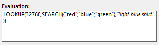
3. Then, the SEARCH function is actually performed on ‘light blue shirt’ for each item in the array, with the result of this in each case either being a number representing the starting position of the array item in the keyword, or a #VALUE! error indicating the item was not found:

So what’s the result of this formula? It’s 7, because of LOOKUP’s special talent – matching the last non-error value.

But ‘7’ isn’t much help in our keyword grouping. Luckily, LOOKUP has another special talent – you can add a ‘result_vector’ range to the end of it, and the value returned will be the item in this range which is in the same order position as the value which LOOKUP matches from the SEARCH array. We haven’t got much time in our example so let’s just use the same range as the lookup_vector that contains the colours:

=LOOKUP(2^15,SEARCH(C2:C4,A2),C2:C4)

Then we lock the ranges (using $) and wrap an iferror around it to tidy it up and hey presto, we have quite possibly the cleverest formula in any digital marketer’s bag of tricks:

=IFERROR(LOOKUP(2^15,SEARCH($C$2:$C$4,A2),$D$2:$D$4),"/")