
Hello, and welcome to my second post in this series, where I dare to stand up against some of the most common Excel challenges we face within this industry, and defeat them head-on with cold, hard, uncompromising logic. You may be well versed in Excel and know much of the below already, but have a look through as I’ll be touching on a number of additional hints and tips along the way as well..
I’ve also attached a worksheet to this post for you to see and work with the examples themselves.
In my previous post I looked at some top tips to save you time in Excel, ranging from data manipulation, to cell formatting and general navigation. In this post I look to tackle the most common uses of the IF statement.
By the way, if you’re a more advanced Excel user and want to explore beyond the IF formula, you may enjoy Found’s latest list of advanced Excel formulas and macros. They will be especially useful if you work in web marketing and regularly handle keyword and URL data, but there’s plenty there for other fields too. Anyway, back to the IFs..
What IF…?
Getting acquainted with the many IF statements will start to open up a whole range of new opportunities for you when you’re looking to analyse and manipulate data. It can be used to quickly fetch results based around given criteria, to sort and catalogue data, or be used in conjunction with other formulas for some very inventive and powerful operations.
The main essence of the statement is to return a result when meeting certain criteria. So for example..
– Return the sum of all clicks IF the month is March
– Return the phrase “Out of Stock” IF the stock level field = 0
– Lookup an associated cost IF a cell contains the word “forecast”
Excel will tell you that the basic IF statement follows this format:
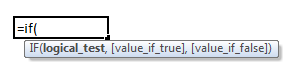
Below I’ve applied this to some very simple statements:
=IF(A1=”March”,1,0)
If the value in cell A1 is equal to “March”, then return a 1, and if it isn’t then return a 0.
=IF(A1>10000,”high spend”,”low spend”)
If the number in cell A1 is greater than £10,000, return “high spend”, and if it isn’t then return “low spend”
Of course you can return more sophisticated results than a simple number or text string if the criteria is met, but we’ll get into those later. Different numerical operators can also be used well in these types of statement. Equal to, Greater than, less than, greater than or equal to etc. can all be used to good effect.
So now the formula is laid down, let’s get into some of these great uses…!
1. Using SumIF, CountIF, and AverageIF
Some of the most common Excel IF formulas allow you to sum, count and average data based on set criteria. To demonstrate these I’ve put together a simple affiliate commission report below:
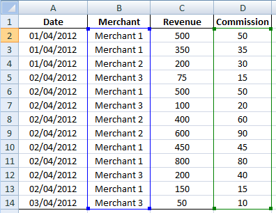
With these particular formulas you first supply the range that you wish to lookup, the criteria that you wish to match in this range, and then finally supply the associated result.
=SUMIF(B2:14,”Merchant 1”,D2:D14)
If column B contains the value “Merchant 1”, return a sum of column D (commission) for that merchant.
=AVERAGEIF(B2:14,”Merchant 1”,D2:D14)
If column B contains the value “Merchant 1”, return an average of column D (commission) for that merchant.
=COUNTIF(B2:14,”Merchant 1”)
If column B contains the value “Merchant 1”, return a count of the number of times it appears.
You won’t always want to apply a text string as the lookup value. In the example below, I wanted to summarise total commission by day and display it in a nice (new) table. You can see I’m looking up the previous data as before, but in this instance I’m summing where the date is equal to the cell next to the formula (F2).
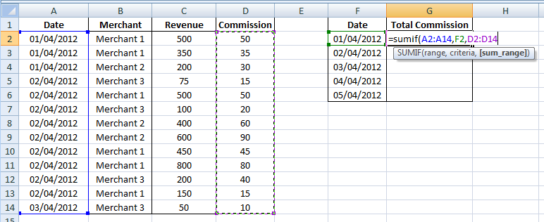
Best Used: When you want to summarise data from a large table, and display it separately.
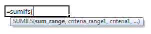
2. Using SumIFs, CountIFs, and AverageIFs
What’s that? You want to do the same thing but with multiple criteria? Well worry not, for the ‘Ifs’ formulas allow you to do just that. Keeping with the previous example, I’ve decided to break my daily commission out even further, and display it by merchant as well. This will give me a more granular overview of performance over time. I’ve adjusted my table so that merchants stretch across the top, with dates going down the side. I’ve also kept both the date format and merchant names exactly the same as in the commission report, so that I can refer to them by cell reference.
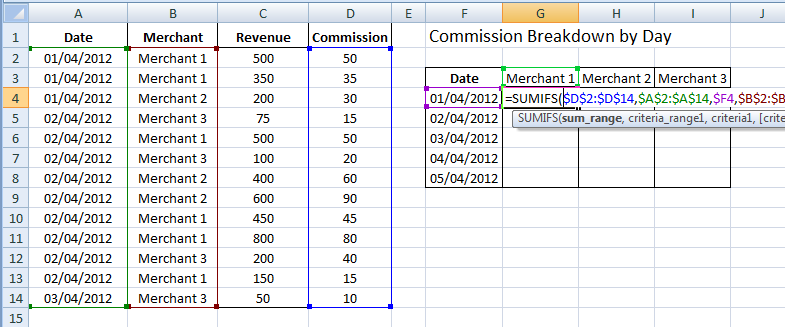
These are slightly different to the previous formulas, as you define the result first, and then supply multiple conditions afterwards..
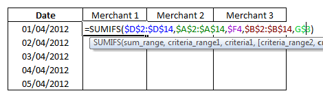
=SUMIFS(D2:D14,A2:A14,F4,B2:B14,G3)
Sum the commission column (D2:D14) where the date column (A2:A14) is equal to the date in my summary table (F4) and the merchant column (B2:B14) is equal to the merchant in my summary table (G3).
It’s worth noting at this stage that my formula makes use of $ symbols as well. These lock cells in place, and stop them updating when you move your formula across. For instance, without $ symbols, my D:D reference would suddenly change to E:E if I moved the formula across one.
You can place $ symbols before both the letter and the number in a cell reference to lock each part individually. Doing it on both will lock the cell, column or row absolutely. If you look at the formula in the table below, you can see I’ve locked the commission table lookups absolutely, but allowed a bit of flexibility with my own table lookups so that the date and merchant update as well. Especially handy if you keep updating the table with new merchants or new dates!
Best Used: When you want to summarise and display data separately, but in a more granular format.
3. IF AND and IF OR
Sometimes there are scenarios where you have very specific criteria that you need to build into your Excel formulas. IF AND can help you define multiple conditions that all need to be met before returning the desired result, and IF OR can return a result when only one of multiple conditions is met.
To put it in the context of another typical, industry scenario..
I’m running a PPC campaign with a bonus scheme set around achieving a set number of sales in a month, and I want to analyse what bonus I’m likely to hit. I’ve started by building out a simple calculator that looks at current sales, and scales it by days in month to bring me an expected sales figure.
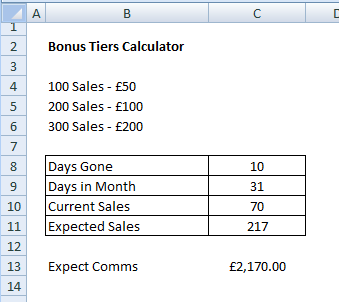
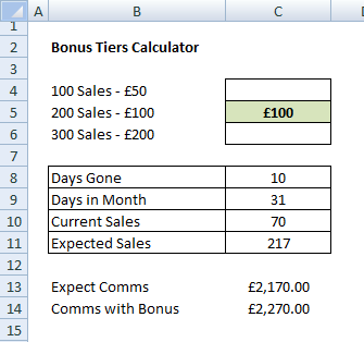
I want the bonus to update automatically throughout the month dependent on expected sales, and add it to the expected commission. There are many ways you can go about doing this, but one particularly tidy example uses IF AND formulas..
To tell if tier 1 has been hit: =IF(AND(C11>99,C11<200),50,””)
If expected sales are greater than 99 and less than 200, return £50 (tier 1) else return nothing.
To tell if tier 2 has been hit: =IF(AND(C11>199,C11<300),100,””)
If expected sales are greater than 199 and less than 300, return £100 (tier 2) else return nothing.
To tell if tier 3 has been hit: =IF(C11>299,200,””)
If expected sales are greater than 299, return £200 (tier 3) else return nothing.
You can build these into a table next to the bonus tiers and include them in a further calculation to show commission with bonus.
The IF OR formula works in much the same way, only with this formula only one of the conditions needs to be true to trigger the output. In the following example I have a breakdown of sales revenue by type of merchant. I want to only calculate revenue for PPC and SEO and display it in a separate column. The IF OR formula can help here..
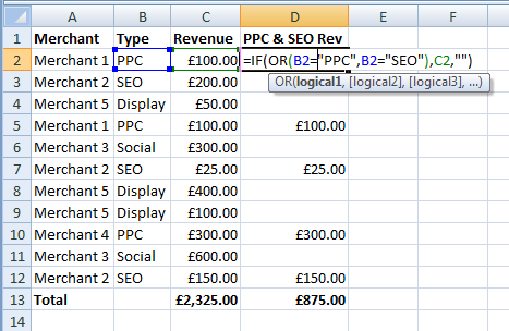
=IF(OR(B2=”PPC”,B2=”SEO”),C2,””)
If cell B2 is equal to PPC or SEO, return the revenue amount, else return nothing.
Best Used: When you want to be a bit more selective with the data you select.
4. Nested Ifs
With Excel, you can actually use the ‘value if false’ option to include further IF statements. If the condition in the first IF formula isn’t met, it will move onto the next IF formula, and so on..
Let’s return to the bonus tier example I gave in point 3. I previously calculated bonus tiers with IF AND statements individually, and returned a number next to them. It looks nice. However if you preferred you could actually scrap this and calculate the whole thing with nested Ifs instead, returning the result in a single cell..
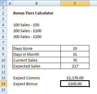
=IF(C11>299,200,(IF(C11>199,100,(IF(C11>99,50,0)))))
If expected sales is greater than 299, return £200 (tier 3) else if expected sales is greater than 199, return £100 (tier 2), else if expected sales is greater than 99, return £50 (tier 1), else return £0.
Note: In this example I had to calculate the tiers in reverse order. If you were to calculate IF sales > 99 in the first IF formula, the condition would be met and it wouldn’t trigger the other IF statements.
Best used: When you want to provide multiple conditions, and return a distinct result for each.
5. Blank out those horrible looking errors with IFERROR
And so on to our final tip for this session, and a really nice formula which can help turn an awful looking table into a much cleaner and more presentable one. I use this formula all the time.
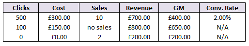
Here is a very simple table that might look quite familiar to you. A simple conversion rate calculation has thrown up two errors. An incorrect entry of “no sales” has forced an incorrect value error, and a ‘divide by 0’ error has been thrown by the last row where there have been 0 clicks.
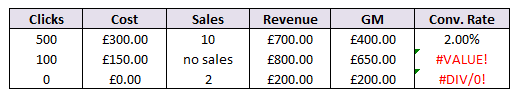
I don’t know about you, but whenever I see these I like to eradicate them upon sight. A simple IFERROR formula appended to your existing formula gives you a lot of control in doing this, and allows you to supply an alternate value.
So where my conversion rate formula previously looked like this:
=(C3/A3)
It now looks a little like this:
=IFERROR((C3/A3), “N/A”)
..where the “N/A” is the value I’ve chosen to replace the error messages.
There. Doesn’t that look better? I’ll be sure to win that client pitch now!
It’s really very simple to apply, and can be used on even the most complicated and long-winded formulas. You can choose anything to replace it with, be it a numerical value, a text value, or even another formula – not bad!
Best used: If you’re sending out data to clients or bosses, and don’t want them sighing in despair.
Stay tuned for yet more Excel blog posts from me in the near future, where I’ll be looking to put even more formulas and shortcuts to good use. Remember to check out the attached worksheet for further info, and my previous post – 5 Great Uses of the 5 Great Time-Saving Excel Tips (you may not know about)