Excel Cheat Sheet for Keyword Marketers

Author

Get domain from URL:

=LEFT(A2,FIND("/",A2,9))

This works by bringing back everything to the left of the first trailing slash found after the initial 2 in ‘http..://’, which in a URL is the slash occurring after the TLD.

Get subdomain from URL:

=IF(SUBSTITUTE(SUBSTITUTE(SUBSTITUTE(SUBSTITUTE(LEFT(A2,FIND(".",A2)),"http://",""),".",""),"https://",""),"domain","")="","none",SUBSTITUTE(SUBSTITUTE(SUBSTITUTE(SUBSTITUTE(LEFT(A2,FIND(".",A2)),"http://",""),".",""),"https://",""),"domain",""))

When you just need the subdomains in a big list from a bunch of differently formatted URLs. This formula works regardless of the presence of the protocol. What it lacks in elegance, it more than makes up for in usefulness.

Remove first X characters from cell:

=RIGHT(A1,LEN(A1)-X)

If there’s something consistent that you want to remove from the front of data in your cells, such as an html tag like <title>, you can use this to remove it by specifying its length in characters in this formula, so X would be 7 in this case.

Remove last X characters from a cell:

=LEFT(B2,LEN(B2)-X)

You might use this to remove the trailing slash from a list of URLs, for example, with X as 1.

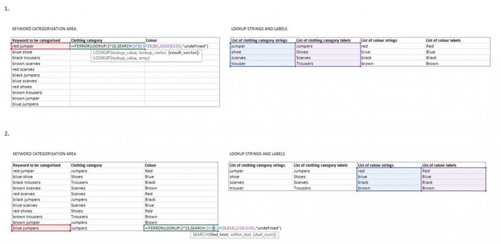
Group keyword phrases automatically based on words they contain:

=IFERROR(LOOKUP(2^15,SEARCH($C$2:$C$200,A2),$D$2:$D$200),"/")

This little chap deserves a blog post all its own – and it got one. Here’s what it does:

Example: Bulk categorisation of keywords by colour and hair type groups.

Using the formula to group your keywords:

1. - $C$2:$C$200 is your string-to-search-for range (the list of all the possible words you want to check for in the keyword).
  - $D$2:$D$200 is your Label to return when string found, put it in the next column along lined up (this can just be the word you’re checking for if you want – same as above)
  - A2 is the cell containing the keyword string which you are searching to see if it contains any of the listed strings so you can label it as such
  - “/” is what gets returned when none of the strings are matched

Word count:

=IF(LEN(TRIM(A2))=0,0,LEN(TRIM(A2))-LEN(SUBSTITUTE(A2," ",""))+1)

See how many words are in your keyword to identify if it’s long tail and get a measure of potential intent.

Find out if a value exists in a range of other values:

=ISNUMBER(MATCH(A2,B:B,0))

This is my favourite, so often we just need to know if URLs in list A are contained within list B. No need to count vlookup columns or iferror. It gives TRUE or FALSE.

Get TRUE or FALSE if a word or string is in a cell:

=ISNUMBER(SEARCH("text-to-find",A2))

If you fancy a break from using the ‘contains’ filter, this can be a way to get things done faster and in a more versatile way.

Remove first word from cell (all before & including 1st space):

=RIGHT(A2,LEN(A2)-FIND(" ",A2))

To remove the last word instead, just use LEFT instead of RIGHT.

Replace the first word in a cell with another word:

=REPLACE(A2,1,LEN(LEFT(A2,FIND(" ",A2)))-1,"X")

“X” is the word you want to replace the incumbent first word with, or this can be a cell reference.

Super trim – more reliable trimming of spaces from cells:

=TRIM(SUBSTITUTE(A2,CHAR(160),CHAR(32)))

Sometimes using =TRIM() fails because of an unconventional space character from something you’ve pasted into Excel. This gets them all.

Perform text-to-columns using a formula:

=TRIM(MID(SUBSTITUTE($A2," ",REPT(" ",LEN($A2))),((COLUMNS($A2:A2)-1)*LEN($A2))+1,LEN($A2)))

This is handy for template building. It provides a way of doing text-to-columns automatically with formulas, using a delimiter you specify. In the example, space ” ” is used as the delimiter.

Extract the final folder path from a URL:

=IF(AND(LEN(A2)-LEN(SUBSTITUTE(A2,"/",""))=3,RIGHT(A2,1)="/"),"",IF(RIGHT(A2,1)="/",RIGHT(LEFT(A2,LEN(A2)-1),LEN(LEFT(A2,LEN(A2)-1))-FIND("@",SUBSTITUTE(LEFT(A2,LEN(A2)-1),"/","@",LEN(LEFT(A2,LEN(A2)-1))-LEN(SUBSTITUTE(LEFT(A2,LEN(A2)-1),"/",""))),1)),RIGHT(A2,LEN(A2)-FIND("@",SUBSTITUTE(A2,"/","@",LEN(A2)-LEN(SUBSTITUTE(A2,"/",""))),1))))

Good for when you need to get just the last portion of a URL, that pertains to the specific page:

Extract the first folder path from a URL:

=IF(LEN(A2)-LEN(SUBSTITUTE(A2,"/",""))>3,LEFT(RIGHT(A2,LEN(A2)-FIND("/",A2,9)),FIND("/",RIGHT(A2,LEN(A2)-FIND("/",A2,9)))-1),RIGHT(A2,LEN(A2)-FIND("/",A2,9)))

Good for extracting language folder.

Remove all text after the Xth instance of a specific character:

=LEFT(A2,FIND(CHAR(160),SUBSTITUTE(A2,"/",CHAR(160),LEN(A2)-LEN(SUBSTITUTE(A2,"/",""))-0)))

Say you want to chop the last folder off a URL, or revert a keyword cluster to a previous hierarchy level. The “/” is the character where the split will occur, change it to whatever you want. The “-0” at the end chops off everything after the last instance. Changing it to -1 would chop off everything after the penultimate instance, and so on.

Create an alphabetical list of column letters for use in other formulas A,B,C…AA,BB etc:

=SUBSTITUTE(ADDRESS(1,ROWS(A$1:A1),4),1,"")

Unlike with numbers, Excel doesn’t automatically give you the next letter of the alphabet if you drag down after selecting cells with ‘a’ and ‘b’ but you can use this to achieve that effect. It runs through the columns, so it will keep working past Z, giving you AA and AB etc. That’s handy for making indirect references in formulas.

Count instances of a character in a cell:

=LEN(A2)-LEN(SUBSTITUTE(A2," ",""))

Countif “*”&”x”&”*” doesn’t cut it for this task because it counts cells, not occurrences. The example here is for ” ” space character.

Count the number of times a specific word appears in a cell:

=(LEN(A2)-LEN(SUBSTITUTE(A2,B2,"")))/LEN(B2)

The formula above works for individual characters, but if you need to count whole words this will work – handy for checking keyword inclusion in landing page copy for SEO. In the example, B2 should contain the word you are counting the instances of within A2.

Return TRUE if there are no numbers in a cell:

=COUNT(FIND({0,1,2,3,4,5,6,7,8,9},B28))<1

Change the end to >0 to show TRUE if there are numbers present. Handy for isolating and removing cells of data which can be identified as unwanted by the presence or absence of a number, such as a mix of item names and item product codes when you only want the item names.

Get the current column letter for use in other formulas:

=MID(ADDRESS(ROW(),COLUMN()),2,SEARCH("$",ADDRESS(ROW(),COLUMN()),2)-2)

If you’re using indirect references and want a fast way to just get the current column letter placed into your formula, use this.

Put your keywords into numbered batches for pulling seasonal search volume data:

=IF(A2=43,1,A2+1)

To save you having to count out 2,500 keywords each time. This batches them up so you just have to filter for the batch number, ctrl A, ctrl C, ctrl V – 43 is the number of keywords in your list divided by 2500, which is the keyword planner limit. Use the blank row insertion macro to make the batches easily selectable.

Word order flipper:

=TRIM(MID(F18,SEARCH(" ",F18)+1,250))&" "&LEFT(F18,SEARCH(" ",F18)-1)

Turns ‘dresses white wedding’ into ‘white wedding dresses’. Use it in steps inside itself to further rearrange words in a different order.

Find the maximum numerical value in a row range, and return the column header:

=INDEX($A$1:$F$1,MATCH(MAX(A2:F2),A2:F2,0))

So if your column headers are months or categories, this brings back which one contains the highest value for that row. Useful for showing which month has the highest search volume for a keyword.

Find position of nth occurrence of character in a cell:

=FIND(CHAR(1),SUBSTITUTE(A1,"c",CHAR(1),3))

Useful as a part of other formulas.

Get all characters after the last instance of a string:

=SUBSTITUTE(RIGHT(A2,LEN(A2)-FIND("@",SUBSTITUTE(A2," > ","@",(LEN(A2)-LEN(SUBSTITUTE(A2," > ","")))/LEN(" > ")))),"> ","")

Gets ‘category 3’ from ‘category 1 > category 2 > category 3’, splitting on the last ‘>’.

Get all characters after the first instance of a string:

=TRIM(MID(A2,SEARCH(" > ",A2)+LEN(" > "),255))

Like the above, but chops off the first category e.g. gets ‘category 2 > category 3’ from ‘category 1 > category 2 > category 3’, splitting on the first ‘>’.

Get URL path from URL in Google Analytics format:

="/"&RIGHT(A2,LEN(A2)-FIND("/",A2,9))

Gets ‘/folder/file’ from ‘https://www.domain.com/folder/file’, I use this to convert URLs to the path format used in Google Analytics exports when I need to vlookup data from the export into another sheet containing full URLs. You could do a find and replace instead, but that doesn’t catch the subdomains and other oddities you may have in your URL list.

Get the next x characters after a string:

This one is cool. If your cell contained ‘product ID:0123 #8392 london’, you could tell this formula to get ‘0123’ based on the presence of ‘product ID:’ in front of it. It says ‘find this, and bring back the next x characters’.

=IFERROR(LEFT(RIGHT(A2,LEN(A2)-(SEARCH("STRING",A2)+6)),6),"")

There are 3 parts you need to change.

Replace STRING with your string to search for e.g. ‘product ID:’
Replace ‘+6’ with the length of your string to search for, so for ‘product ID:’ it would be ‘+11’
Replace the next number, ‘6’, with the number of characters you want to capture after the end of the string to search for. So to capture ‘0123’ from ‘product ID:0123’ you’d put ‘4’.

=IFERROR(LEFT(RIGHT(A2,LEN(A2)-(SEARCH("product ID:",A2)+11)),4),"")

So it’s a bit like regex capture. I used this to get the width and height of images in raw HTML.

Identify cells containing non-alphanumeric characters

This returns TRUE if your cell contains any character which is not a number or letter. It’s great for weeding out the mis-spelled junk keywords from Google Search Console, like ‘blue tango shoes.’ and ‘/blue tango shoes’

=ISERR(SUMPRODUCT(SEARCH(MID(A2,ROW(INDIRECT("1:"&LEN(A2))),1),"abcdefghijklmnopqrstuvwxyz 1234567890-")))

It returns TRUE if it finds anything that is not x, where x is the characters in the quotes at the end. You can modify this, for example, to return TRUE if it finds numbers by deleting the numbers from between the quotes. For reasons that are beyond me, it doesn’t identify question marks.

Capitalise only the first letter in a cell

Excel’s ribbon can can capitalise all characters in a cell with UPPER, or the first of each word with PROPER. But what if you just want the very first letter of the cell capitalised? This will do what you need:

=REPLACE(LOWER(A2),1,1,UPPER(LEFT(A2,1)))

It’s especially handy for getting lowercase metadata ready for upload.

EXCEL VBA MODULES

VBA does stuff to your spreadsheets by pressing a button. Usually this is stuff that would take a long time to do (or be hard / impossible to do) using the normal Excel ribbon & formula capabilities.

To use these:

1. 1. Save your workbook as .xlsm
  2. Reopen it and hit alt + f11
  3. In the menu, insert > module
  4. Paste in the code
  5. Press the play button

There’s no need to understand the code. But be careful to save a backup copy of your workbook before running any of these – they can’t be undone with ctrl + z!

Convert all non-clickable URLs in your spreadsheet to clickable hyperlinks:

So you can visit the URLs easily if you need to e.g. for optimisation of a lot of pages, so you don’t have to mess about double clicking each one to get it ready.

Sub HyperAdd()

For Each xCell In Selection
 ActiveSheet.Hyperlinks.Add Anchor:=xCell, Address:=xCell.Formula
 Next xCell

End Sub

Conditional formatting by row value:

So the colour intensity is relative to each row only, rather than the entire range. You need to use this to complete the search landscape document seasonality tab.

Sub NewCF()
 Range("B1:P1").Copy
 For Each r In Selection.Rows
 r.PasteSpecial (xlPasteFormats)
 Next r
 Application.CutCopyMode = False
 End Sub

Remove duplicates individually by column:

If you have a lot of columns, each of which needs duplicates removing individually e.g. if you have a series of category taxonomies to clean – you can’t do this from the menu:

Sub removeDups()
 Dim col As Range
 For Each col In Range("A:Z").Columns
 With col
 .RemoveDuplicates Columns:=1, Header:=xlYes
 End With
 Next col
 End Sub

Merge adjacent cells in a range based on identical value:

To save you doing it individually when you need to make a spreadsheet look good:

Sub MergeSameCell()
 'Updateby20131127
 Dim Rng As Range, xCell As Range
 Dim xRows As Integer
 xTitleId = "KutoolsforExcel"
 Set WorkRng = Application.Selection
 Set WorkRng = Application.InputBox("Range", xTitleId, WorkRng.Address, Type:=8)
 Application.ScreenUpdating = False
 Application.DisplayAlerts = False
 xRows = WorkRng.Rows.Count
 For Each Rng In WorkRng.Columns
 For i = 1 To xRows - 1
 For j = i + 1 To xRows
 If Rng.Cells(i, 1).Value <> Rng.Cells(j, 1).Value Then
 Exit For
 End If
 Next
 WorkRng.Parent.Range(Rng.Cells(i, 1), Rng.Cells(j - 1, 1)).Merge
 i = j - 1
 Next
 Next
 Application.DisplayAlerts = True
 Application.ScreenUpdating = True
 End Sub

Remove all instances of any text between and including 2 characters from a cell (in this example, the < and >):

Especially good for removing HTML tags from screaming frog extractions, kind of a stand in for regex.

Public Function DELBRC(ByVal str As String) As String
 While InStr(str, "<") > 0 And InStr(str, ">") > InStr(str, "<")
 str = Left(str, InStr(str, "<") - 1) & Mid(str, InStr(str, ">") + 1)
 Wend
 DELBRC = Trim(str)
 End Function

Highlight mis-spelled words:

This can help you identify garbled / nonsense keywords from a large set, or just to spellcheck in Excel if you need to.

Sub Highlight_Misspelled_Words()
 For Each cell In ActiveSheet.UsedRange
 If Not Application.CheckSpelling(Word:=cell.Text) Then cell.Interior.ColorIndex = 3
 Next
 End Sub

Lock all slicers in position:

If you send Excel documents to clients with slicers in them, you might worry that they’ll end up moving the slicers around while trying to use them – a poor experience which makes your document feel less professional. But there’s a way around it – run this code and your slicers will be locked in place across all worksheets, while still operational. This effect persists when the document is re-saved as a normal .xlsx file.

Option Explicit

Sub DisableAllSlicersMoveAndResize()

 Dim oSlicerCache As SlicerCache
 Dim oSlicer As Slicer
 
 For Each oSlicerCache In ActiveWorkbook.SlicerCaches
 For Each oSlicer In oSlicerCache.Slicers
 oSlicer.DisableMoveResizeUI = True
 Next oSlicer
 Next oSlicerCache
 
End Sub

Split delimited values in a cell into multiple rows with key column retained:

It’s easy to put a delimited string (Keyword,Volume,CPC…) into columns using text-to-columns but what if you want it split vertically instead, into rows? This can help:

Sub SliceNDice()
 Dim objRegex As Object
 Dim X
 Dim Y
 Dim lngRow As Long
 Dim lngCnt As Long
 Dim tempArr() As String
 Dim strArr
 Set objRegex = CreateObject("vbscript.regexp")
 objRegex.Pattern = "^\s+(.+?)$"
 'Define the range to be analysed
 X = Range([a1], Cells(Rows.Count, "b").End(xlUp)).Value2
 ReDim Y(1 To 2, 1 To 1000)
 For lngRow = 1 To UBound(X, 1)
 'Split each string by ","
 tempArr = Split(X(lngRow, 2), ",")
 For Each strArr In tempArr
 lngCnt = lngCnt + 1
 'Add another 1000 records to resorted array every 1000 records
 If lngCnt Mod 1000 = 0 Then ReDim Preserve Y(1 To 2, 1 To lngCnt + 1000)
 Y(1, lngCnt) = X(lngRow, 1)
 Y(2, lngCnt) = objRegex.Replace(strArr, "$1")
 Next
 Next lngRow
 'Dump the re-ordered range to columns C:D
 [c1].Resize(lngCnt, 2).Value2 = Application.Transpose(Y)
 End Sub

Make multiple copies of a worksheet at once:

If you are making a reporting template for example, and want to get the sheets for all 12 weeks created in one go:

Sub swtbeb4lyfe43()

ThisWS = "name-of-existing-worksheet"
 '# of new sheets
 s = 6
 '# of new sheets
 For i = 2 To s
 Worksheets("name-of-existing-worksheet-ending-with-1").Copy After:=Worksheets(Worksheets.Count)
 ActiveSheet.Name = ThisWS & i
 Next i
 End Sub

Add a specific number of new rows based on cell value:

Saves repeatedly using insert row, pressing F4 etc:

Sub test()
 On Error Resume Next
 For r = Cells(Rows.Count, "E").End(xlUp).Row To 2 Step -1
 For rw = 2 To Cells(r, "E").Value + 1
 Cells(r + 1, "E").EntireRow.Insert
 Next rw, r
 End Sub

Column stacker:

This one’s great when you have lots of columns of information that you want to be combined all into one master column:

Sub ConvertRangeToColumn()
 'UpdatebyExtendoffice
 Dim Range1 As Range, Range2 As Range, Rng As Range
 Dim rowIndex As Integer
 xTitleId = "KutoolsforExcel"
 Set Range1 = Application.Selection
 Set Range1 = Application.InputBox("Source Ranges:", xTitleId, Range1.Address, Type:=8)
 Set Range2 = Application.InputBox("Convert to (single cell):", xTitleId, Type:=8)
 rowIndex = 0
 Application.ScreenUpdating = False
 For Each Rng In Range1.Rows
 Rng.Copy
 Range2.Offset(rowIndex, 0).PasteSpecial Paste:=xlPasteAll, Transpose:=True
 rowIndex = rowIndex + Rng.Columns.Count
 Next
 Application.CutCopyMode = False
 Application.ScreenUpdating = True
 End Sub

Superfast find and replace for huge datasets:

To match partial cell, change to ‘X1Part”.

Sub Macro1()

Application.EnableEvents = False
 Application.ScreenUpdating = False
 Application.Calculation = xlCalculationManual

' fill your range in here
 Range("S2:AJ252814").Select
 ' choose what to search for and what to replace with here
 Selection.Replace What:="0", Replacement:="/", LookAt:=xlWhole, SearchOrder:=xlByRows, MatchCase:=False, SearchFormat:=False, ReplaceFormat:=False

Application.EnableEvents = True
 Application.ScreenUpdating = True
 Application.Calculation = xlCalculationAutomatic
 Application.CalculateFull

End Sub

Paste all cells as values in a worksheet in the active range:

For when your spreadsheet is too slow to do it manually

Sub ToVals()
 With ActiveSheet.UsedRange
 .Value = .Value
 End With
 End Sub

Format all cells to general format or whatever you like, without having to select them:

Another good one for when your spreadsheet is too slow.

Sub dural()
 ActiveSheet.Cells.NumberFormat = "General"
 End Sub

Formula activation – Insert equals at the beginning for a range of cells:

If you’re making something complex with a lot of formulas that you don’t want switched on yet, but you want to be able to use other formulas at the same time (i.e. can’t turn off calculations) this can help. It’s also good for just adding things to the start of cells:

Sub Insert_Equals()

Application.ScreenUpdating = False

Dim cell As Range

For Each cell In Selection
 cell.Formula = "=" & cell.Value
 Next cell

Application.ScreenUpdating = True

End Sub

Consolidate all worksheets from multiple workbooks in a folder on your computer into a single workbook with all the worksheets added into it:

If you have a big collection of workbooks which you want consolidated into one, you can do it in a single step using this macro. Especially good for when the workbooks you need to consolidate are big and slow.

Sub CombineFiles()

Dim Path As String
 Dim FileName As String
 Dim Wkb As Workbook
 Dim WS As Worksheet

Application.EnableEvents = False
 Application.ScreenUpdating = False
 Path = "C:\scu" 'Change as needed
 FileName = Dir(Path & "\*.xl*", vbNormal)
 Do Until FileName = ""
 Set Wkb = Workbooks.Open(FileName:=Path & "\" & FileName)
 For Each WS In Wkb.Worksheets
 WS.Copy After:=ThisWorkbook.Sheets(ThisWorkbook.Sheets.Count)
 Next WS
 Wkb.Close False
 FileName = Dir()
 Loop
 Application.EnableEvents = True
 Application.ScreenUpdating = True

End Sub

Fast deletion of named columns in a spreadsheet which is responding slowly:

Sometimes, one does not simply ‘delete a column’. This is for those times.

Sub Delete_Surplus_Columns()

Dim FindString As String
 Dim iCol As Long, LastCol As Long, FirstCol As Long
 Dim CalcMode As Long

With Application
 CalcMode = .Calculation
 .Calculation = xlCalculationManual
 .ScreenUpdating = False
 End With

FirstCol = 1
 With ActiveSheet
 .DisplayPageBreaks = False

LastCol = .Cells(3, Columns.Count).End(xlToLeft).Column

For iCol = LastCol To FirstCol Step -1

If IsError(.Cells(3, iCol).Value) Then
 'Do nothing
 'This avoids an error if there is a error in the cell
 ElseIf .Cells(3, iCol).Value = "Value B" Then
 .Columns(iCol).Delete
 ElseIf .Cells(3, iCol).Value = "Value C" Then
 .Columns(iCol).Delete
 End If

Next iCol

End With

With Application
 .ScreenUpdating = True
 .Calculation = CalcMode
 End With

End Sub

Find and replace based on a table in another worksheet:

Use X1Part for string match & replace within a cell, or X1 whole for whole cell match & replace:

Sub Substitutions()

Dim rngData As Range
 Dim rngLookup As Range
 Dim Lookup As Range

With Sheets("Sheet1")
 Set rngData = .Range("A1", .Range("A" & Rows.Count).End(xlUp))
 End With

With Sheets("Sheet2")
 Set rngLookup = .Range("A1", .Range("A" & Rows.Count).End(xlUp))
 End With

For Each Lookup In rngLookup
 If Lookup.Value <> "" Then
 rngData.Replace What:=Lookup.Value, _
 Replacement:=Lookup.Offset(0, 1).Value, _
 LookAt:=xlWhole, _
 SearchOrder:=xlByRows, _
 MatchCase:=False
 End If
 Next Lookup

End Sub

Unhide all sheets in a workbook:

Do your hidden sheets tell the tale of 1,000 previous clients? You don’t need me to tell you this can look unprofessional. Bring those hidden sheets up from the dregs in one go with this vba code so you can delete them. Otherwise, you’ll have to tediously unhide them 1 by 1 – there is no option in the interface to do this all at once.

Sub Unhide_All_Sheets()
    Dim wks As Worksheet
     For Each wks In ActiveWorkbook.Worksheets
        wks.Visible = xlSheetVisible
    Next wks
End Sub

Change pivot table data source for all pivot tables on a worksheet:

Your data source has changed. You have 12 pivot tables to update. You just lost your lunch break. Or did you? To update all their data sources in one fell swoop, replace WORKSHEETNAME with the name of your worksheet and DATA with the name of your data source:

Sub Change_Pivot_Source()
    Dim pt As PivotTable
    For Each pt In ActiveWorkbook.Worksheets("WORKSHEETNAME").PivotTables
             pt.ChangePivotCache ActiveWorkbook.PivotCaches.Create _
                (SourceType:=xlDatabase, SourceData:="DATA")
    Next pt
End Sub

Convert all ‘numbers stored as text’ to general:

“Number stored as text!” .We’ve all seen it. We’ve all been annoyed by it. I had several thousand rows to convert and this took minutes, not seconds.

Skip it all using this, replacing your range:

Sub macro()
Range("AG:AK").Select 'specify the range which suits your purpose
With Selection
Selection.NumberFormat = "general"
.Value = .Value
End With
End Sub

There are other ways to do it, but if you have a big dataset, this is the fastest way.

BONUS TIPS

1. - If you have a slow spreadsheet that’s locked up Excel while it’s calculating, but you still need to use Excel for other stuff, you can open a completely new instance of Excel by holding Alt, clicking Excel in the taskbar, and answering ‘yes’ to the pop up box. This isn’t just a new worksheet – it’s a totally new instance of Excel.
  - To open a new workbook in the same instance of Excel a bit more quickly than usual when you already have workbooks open, you can use a single middle mouse click on Excel in the taskbar.

We’ve written some other blog posts about excel, you can find them here:

- 5 GREAT USES OF THE IF FORMULA IN EXCEL (YOU MAY NOT KNOW ABOUT)
- 5 GREAT TIME-SAVING EXCEL TIPS (YOU MAY NOT KNOW ABOUT)

Suggested

Exploring New Horizons in Social Media Platforms

Jamie Klingler explores new social media platform Blue Sky and shares her thoughts on this new horizon in social media.

Jamie Klingler, 19 Nov 2024

Everything is Influenced

Stevie Johnson, MD of Disrupt (Found’s sister company), delves into the ever evolving landscape of influencer marketing at Web Summit.

Rachel Leamon, 15 Nov 2024